Stack overlapping objects on top of one another.

position_fill additionally standardises each stack to have unit height.

Usage

position_fill()

position_stack()

See also

See geom_bar and geom_area for more examples.

Other position adjustments: position_dodge(), position_identity(), position_jitter(), position_jitterdodge(), position_nudge()

Examples

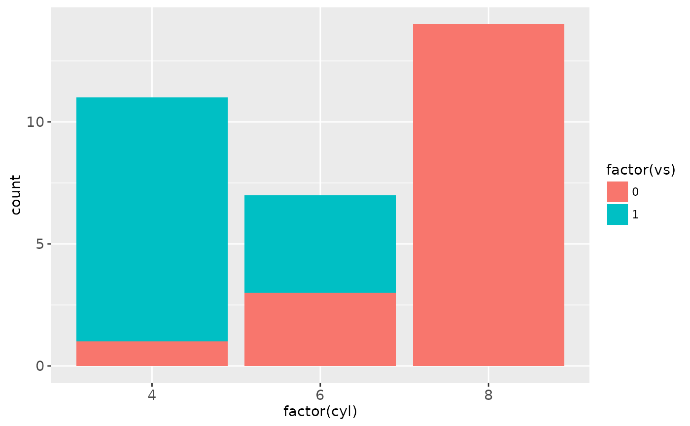
# Stacking is the default behaviour for most area plots:
ggplot(mtcars, aes(factor(cyl), fill = factor(vs))) + geom_bar()

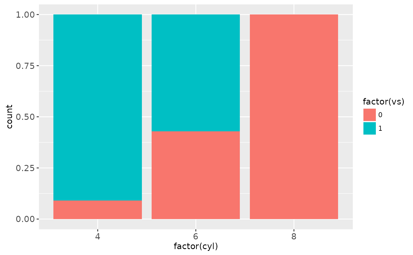
# Fill makes it easier to compare proportions
ggplot(mtcars, aes(factor(cyl), fill = factor(vs))) +
  geom_bar(position = "fill")


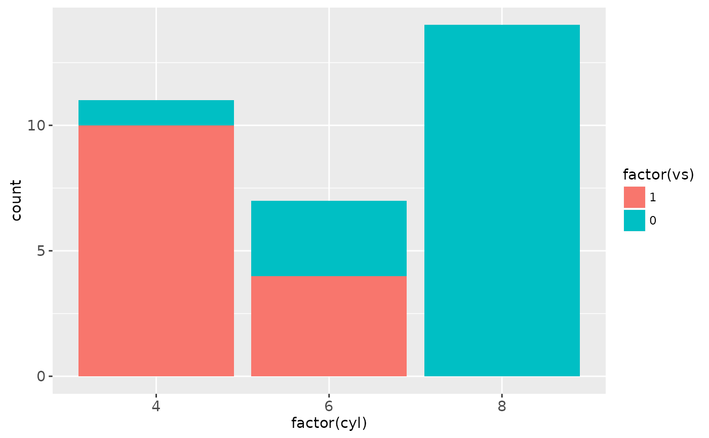
# To change stacking order, use factor() to change order of levels
mtcars$vs <- factor(mtcars$vs, levels = c(1,0))
ggplot(mtcars, aes(factor(cyl), fill = factor(vs))) + geom_bar()


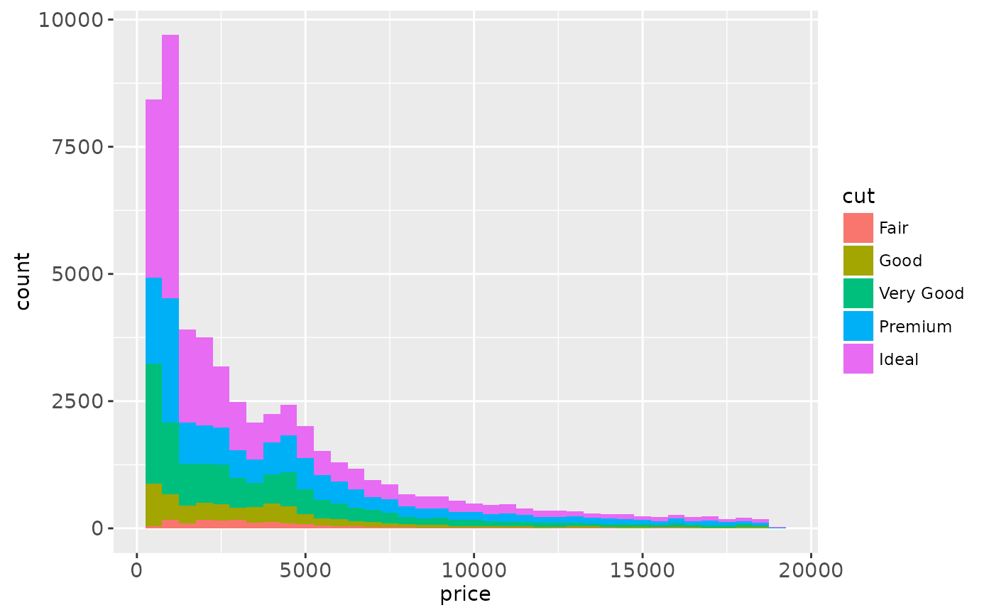
ggplot(diamonds, aes(price, fill = cut)) +
  geom_histogram(binwidth = 500)

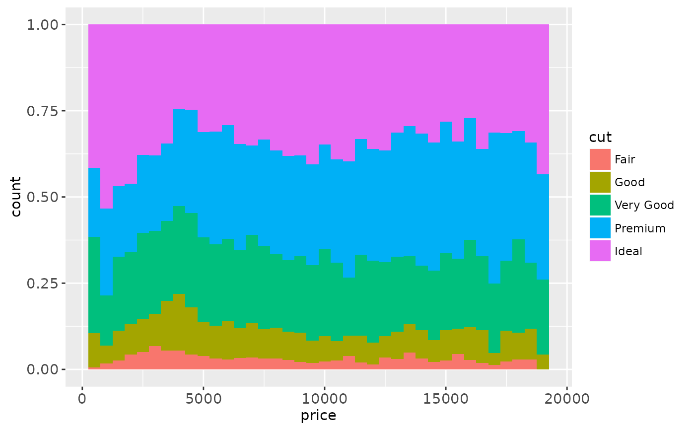
# When used with a histogram, position_fill creates a conditional density
# estimate
ggplot(diamonds, aes(price, fill = cut)) +
  geom_histogram(binwidth = 500, position = "fill")


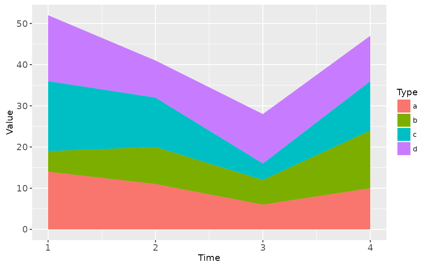
# Stacking is also useful for time series
data.set <- data.frame(
  Time = c(rep(1, 4),rep(2, 4), rep(3, 4), rep(4, 4)),
  Type = rep(c('a', 'b', 'c', 'd'), 4),
  Value = rpois(16, 10)
)

ggplot(data.set, aes(Time, Value)) + geom_area(aes(fill = Type))


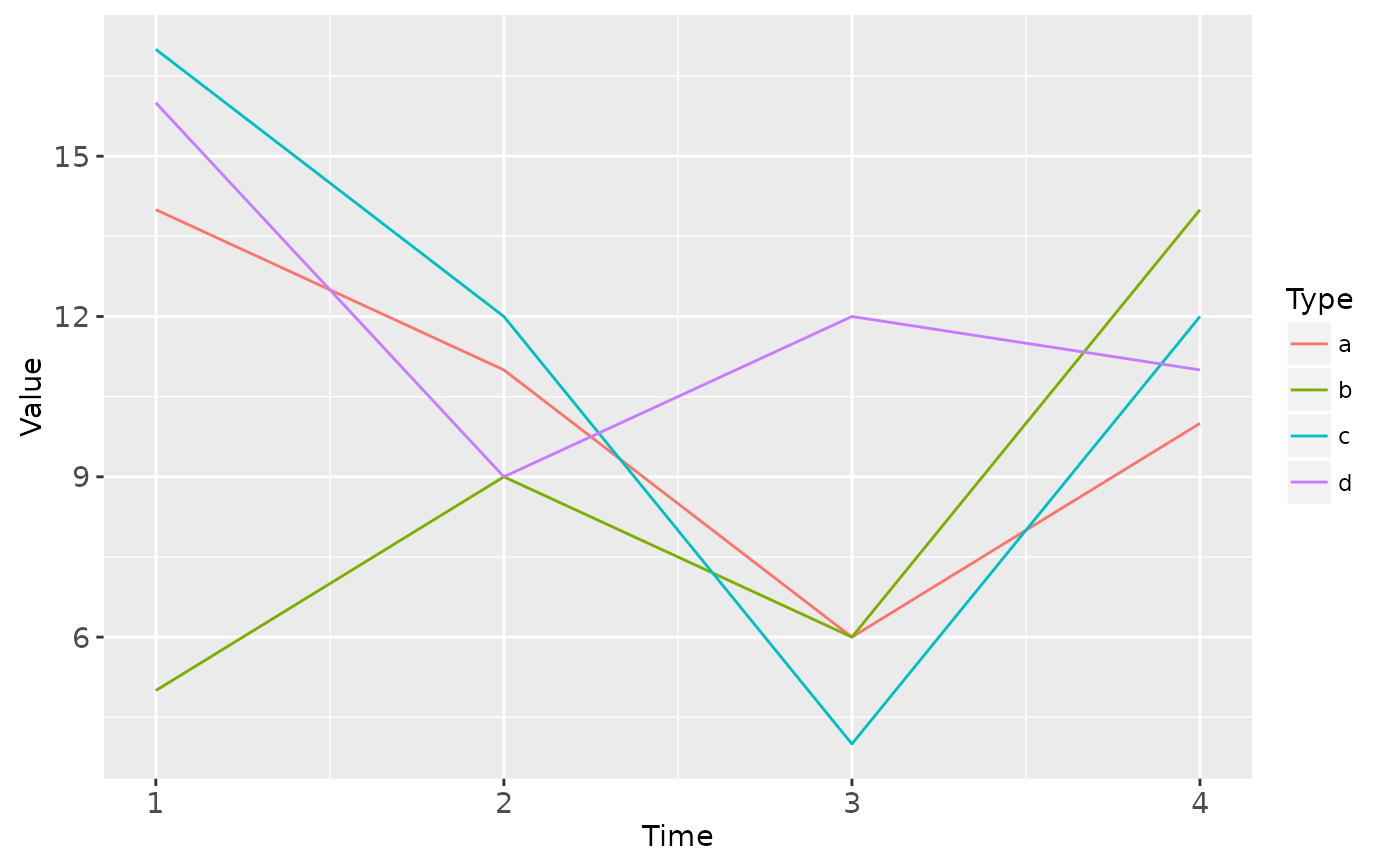
# If you want to stack lines, you need to say so:
ggplot(data.set, aes(Time, Value)) + geom_line(aes(colour = Type))

ggplot(data.set, aes(Time, Value)) +
  geom_line(position = "stack", aes(colour = Type))


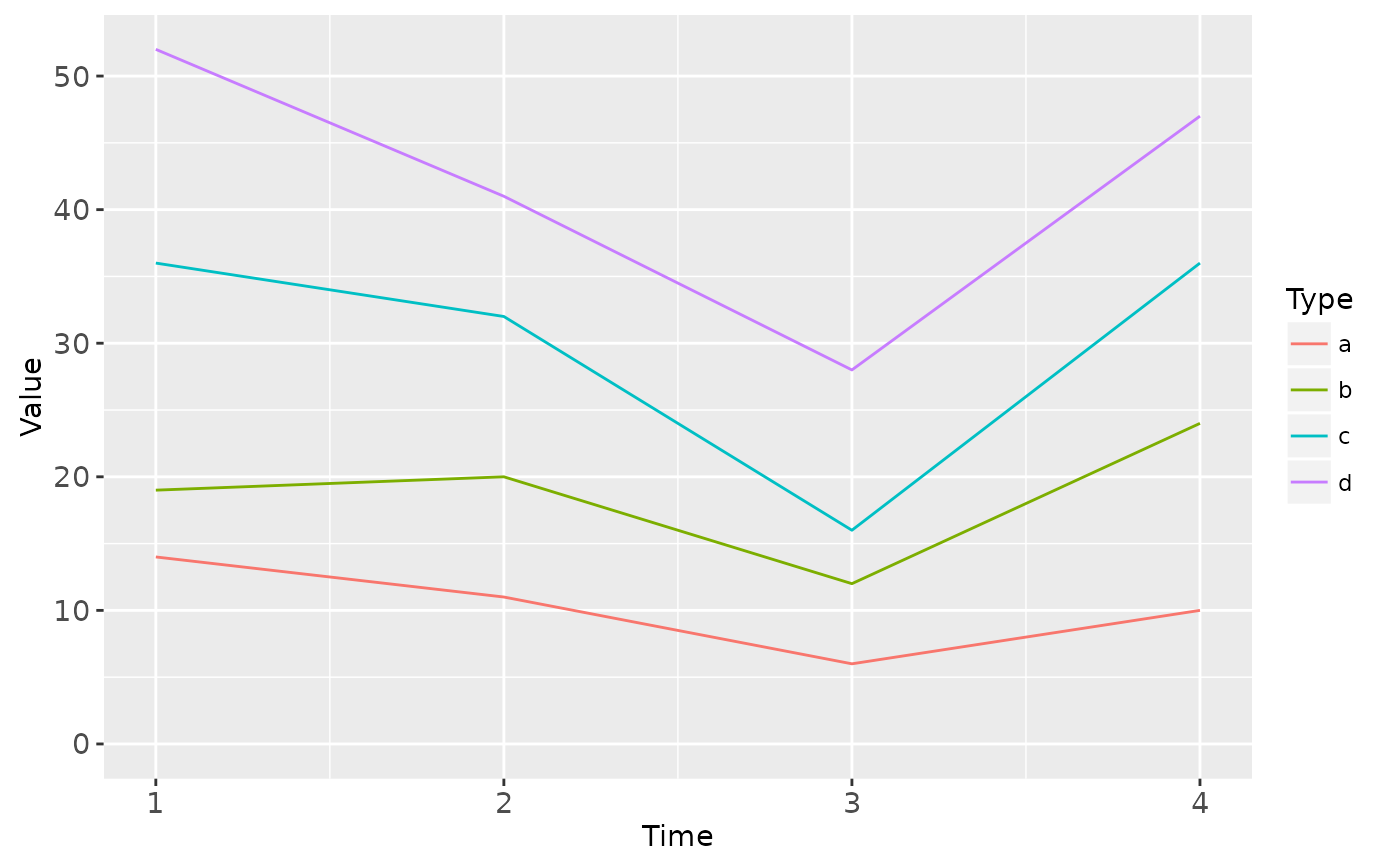# But realise that this makes it *much* harder to compare individual
# trends