Count the number of observations at each location.
Source:R/geom-count.r, R/stat-sum.r
geom_count.RdThis is a variant geom_point that counts the number of
observations at each location, then maps the count to point size. It
useful when you have discrete data.
Usage
geom_count(
  mapping = NULL,
  data = NULL,
  stat = "sum",
  position = "identity",
  ...,
  na.rm = FALSE,
  show.legend = NA,
  inherit.aes = TRUE
)

stat_sum(
  mapping = NULL,
  data = NULL,
  geom = "point",
  position = "identity",
  ...,
  na.rm = FALSE,
  show.legend = NA,
  inherit.aes = TRUE
)
Arguments
- mapping
Set of aesthetic mappings created by
aesoraes_. If specified andinherit.aes = TRUE(the default), it is combined with the default mapping at the top level of the plot. You must supplymappingif there is no plot mapping.- data
The data to be displayed in this layer. There are three options:
If
NULL, the default, the data is inherited from the plot data as specified in the call toggplot.A
data.frame, or other object, will override the plot data. All objects will be fortified to produce a data frame. Seefortifyfor which variables will be created.A
functionwill be called with a single argument, the plot data. The return value must be adata.frame., and will be used as the layer data.- position
Position adjustment, either as a string, or the result of a call to a position adjustment function.
- ...
other arguments passed on to
layer. These are often aesthetics, used to set an aesthetic to a fixed value, likecolor = "red"orsize = 3. They may also be parameters to the paired geom/stat.- na.rm
If
FALSE(the default), removes missing values with a warning. IfTRUEsilently removes missing values.- show.legend
logical. Should this layer be included in the legends?
NA, the default, includes if any aesthetics are mapped.FALSEnever includes, andTRUEalways includes.- inherit.aes
If
FALSE, overrides the default aesthetics, rather than combining with them. This is most useful for helper functions that define both data and aesthetics and shouldn't inherit behaviour from the default plot specification, e.g.borders.- geom, stat
Use to override the default connection between
geom_countandstat_sum.
Aesthetics
geom_point understands the following aesthetics (required aesthetics are in bold):
x
y
alpha
colour
fill
shape
size
stroke
Computed variables
- n
number of observations at position
- prop
percent of points in that panel at that position
Examples
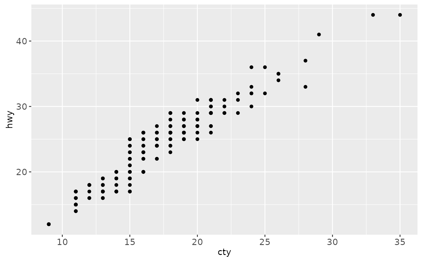
ggplot(mpg, aes(cty, hwy)) +
geom_point()
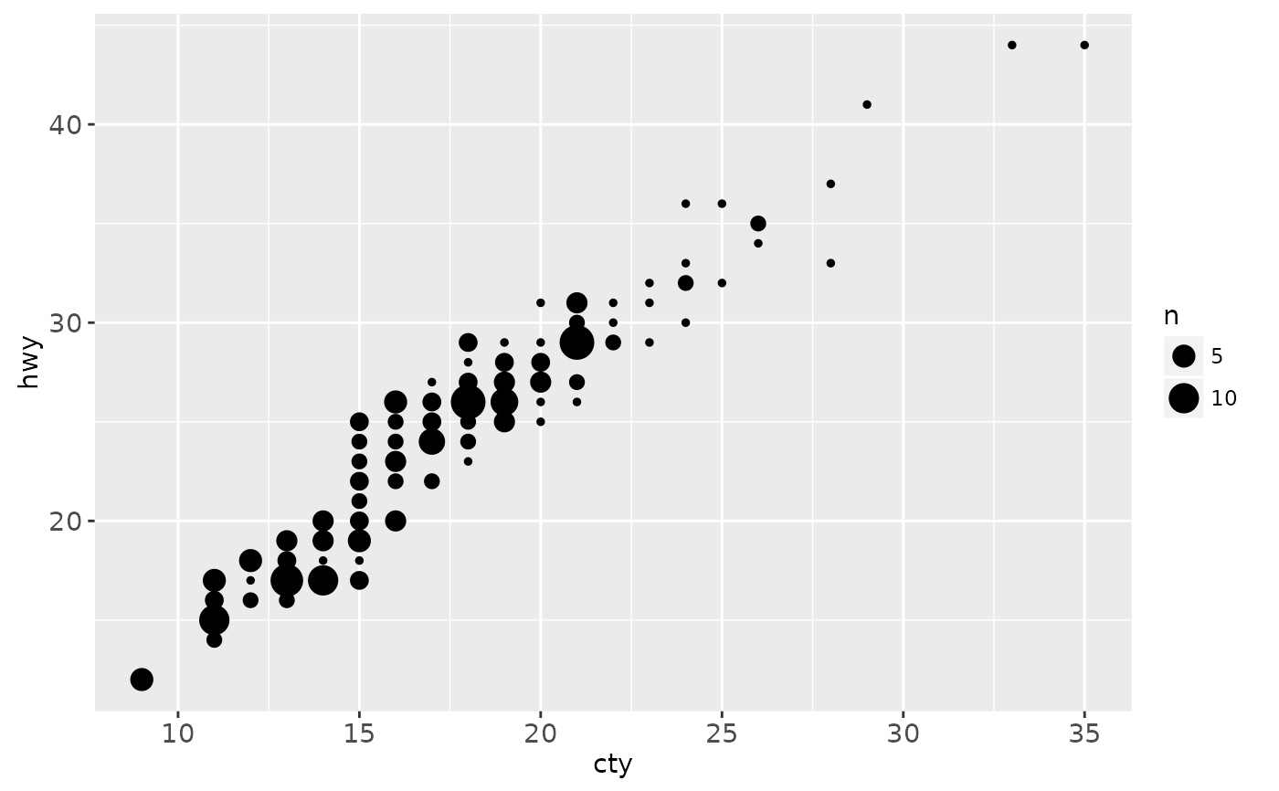
 ggplot(mpg, aes(cty, hwy)) +
geom_count()
ggplot(mpg, aes(cty, hwy)) +
geom_count()
 # Best used in conjunction with scale_size_area which ensures that
# counts of zero would be given size 0. Doesn't make much different
# here because the smallest count is already close to 0.
ggplot(mpg, aes(cty, hwy)) +
geom_count()
# Best used in conjunction with scale_size_area which ensures that
# counts of zero would be given size 0. Doesn't make much different
# here because the smallest count is already close to 0.
ggplot(mpg, aes(cty, hwy)) +
geom_count()
 scale_size_area()
#> <ScaleContinuous>
#> Range:
#> Limits: 0 -- 1
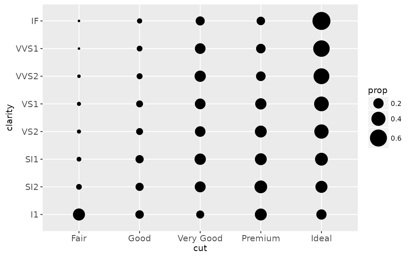
# Display proportions instead of counts -------------------------------------
# By default, all categorical variables in the plot form the groups.
# Specifying geom_count without a group identifier leads to a plot which is
# not useful:
d <- ggplot(diamonds, aes(x = cut, y = clarity))
d + geom_count(aes(size = ..prop..))
scale_size_area()
#> <ScaleContinuous>
#> Range:
#> Limits: 0 -- 1
# Display proportions instead of counts -------------------------------------
# By default, all categorical variables in the plot form the groups.
# Specifying geom_count without a group identifier leads to a plot which is
# not useful:
d <- ggplot(diamonds, aes(x = cut, y = clarity))
d + geom_count(aes(size = ..prop..))
 # To correct this problem and achieve a more desirable plot, we need
# to specify which group the proportion is to be calculated over.
d + geom_count(aes(size = ..prop.., group = 1)) +
scale_size_area(max_size = 10)
# To correct this problem and achieve a more desirable plot, we need
# to specify which group the proportion is to be calculated over.
d + geom_count(aes(size = ..prop.., group = 1)) +
scale_size_area(max_size = 10)
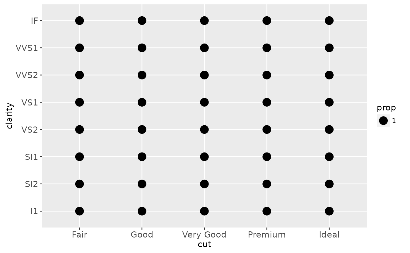
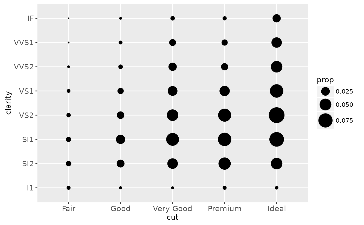 # Or group by x/y variables to have rows/columns sum to 1.
d + geom_count(aes(size = ..prop.., group = cut)) +
scale_size_area(max_size = 10)
# Or group by x/y variables to have rows/columns sum to 1.
d + geom_count(aes(size = ..prop.., group = cut)) +
scale_size_area(max_size = 10)
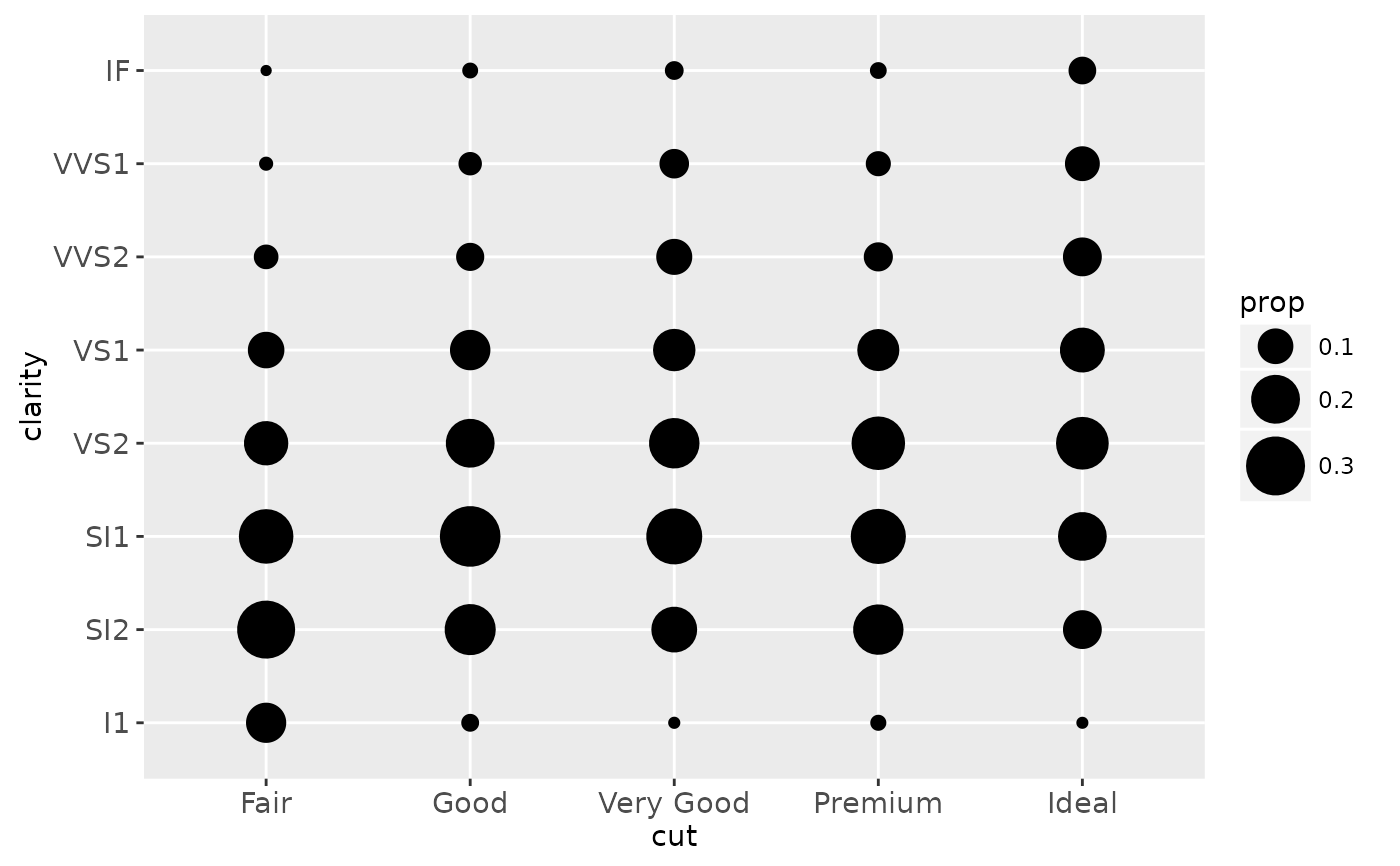 d + geom_count(aes(size = ..prop.., group = clarity)) +
scale_size_area(max_size = 10)
d + geom_count(aes(size = ..prop.., group = clarity)) +
scale_size_area(max_size = 10)