Wrap a 1d ribbon of panels into 2d. — facet

Most displays are roughly rectangular, so if you have a categorical variable with many levels, it doesn't make sense to try and display them all in one row (or one column). To solve this dilemma, facet_wrap wraps a 1d sequence of panels into 2d, making best use of screen real estate.

Usage

facet_wrap(
  facets,
  nrow = NULL,
  ncol = NULL,
  scales = "fixed",
  shrink = TRUE,
  labeller = "label_value",
  as.table = TRUE,
  switch = NULL,
  drop = TRUE,
  dir = "h"
)

Arguments

facets: Either a formula or character vector. Use either a one sided formula, ~a + b, or a character vector, c("a", "b").
nrow, ncol: Number of rows and columns.
scales: should Scales be fixed ("fixed", the default), free ("free"), or free in one dimension ("free_x", "free_y").
shrink: If TRUE, will shrink scales to fit output of statistics, not raw data. If FALSE, will be range of raw data before statistical summary.
labeller: A function that takes one data frame of labels and returns a list or data frame of character vectors. Each input column corresponds to one factor. Thus there will be more than one with formulae of the type ~cyl + am. Each output column gets displayed as one separate line in the strip label. This function should inherit from the "labeller" S3 class for compatibility with labeller(). See label_value for more details and pointers to other options.
as.table: If TRUE, the default, the facets are laid out like a table with highest values at the bottom-right. If FALSE, the facets are laid out like a plot with the highest value at the top-right.
switch: By default, the labels are displayed on the top of the plot. If switch is "x", they will be displayed to the bottom. If "y", they will be displayed to the left, near the y axis.
drop: If TRUE, the default, all factor levels not used in the data will automatically be dropped. If FALSE, all factor levels will be shown, regardless of whether or not they appear in the data.
dir: Direction: either "h" for horizontal, the default, or "v", for vertical.

Examples

ggplot(mpg, aes(displ, hwy)) +
  geom_point() +
  facet_wrap(~class)


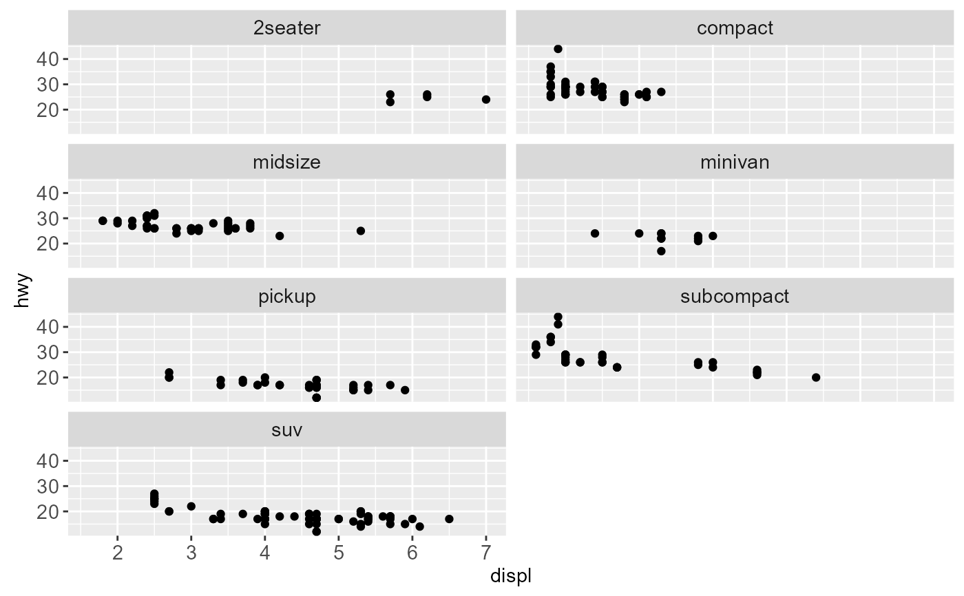
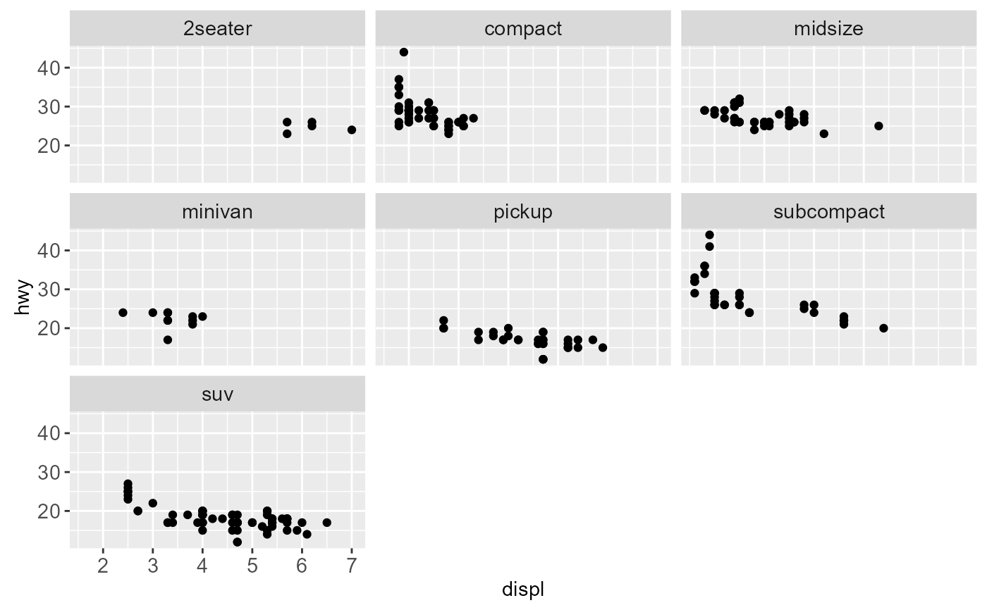# Control the number of rows and columns with nrow and ncol
ggplot(mpg, aes(displ, hwy)) +
  geom_point() +
  facet_wrap(~class, nrow = 4)


# \donttest{
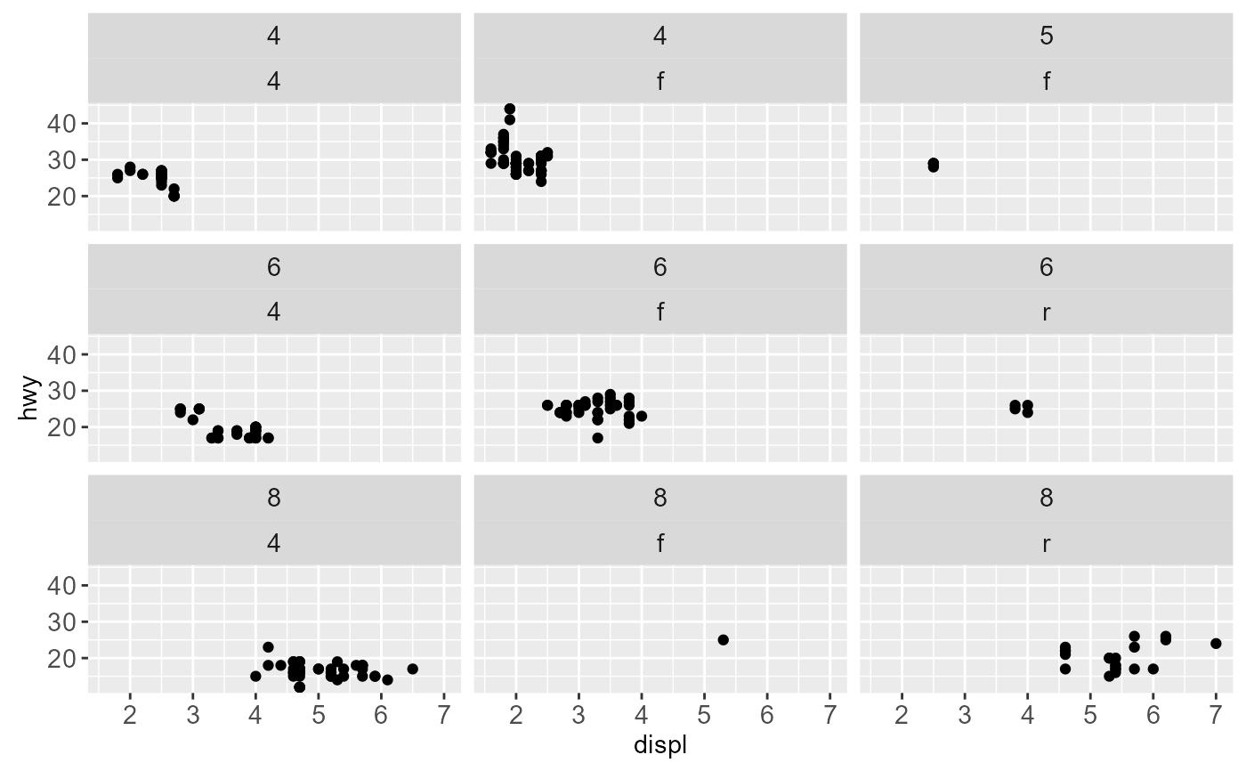
# You can facet by multiple variables
ggplot(mpg, aes(displ, hwy)) +
  geom_point() +
  facet_wrap(~ cyl + drv)

# Or use a character vector:
ggplot(mpg, aes(displ, hwy)) +
  geom_point() +
  facet_wrap(c("cyl", "drv"))


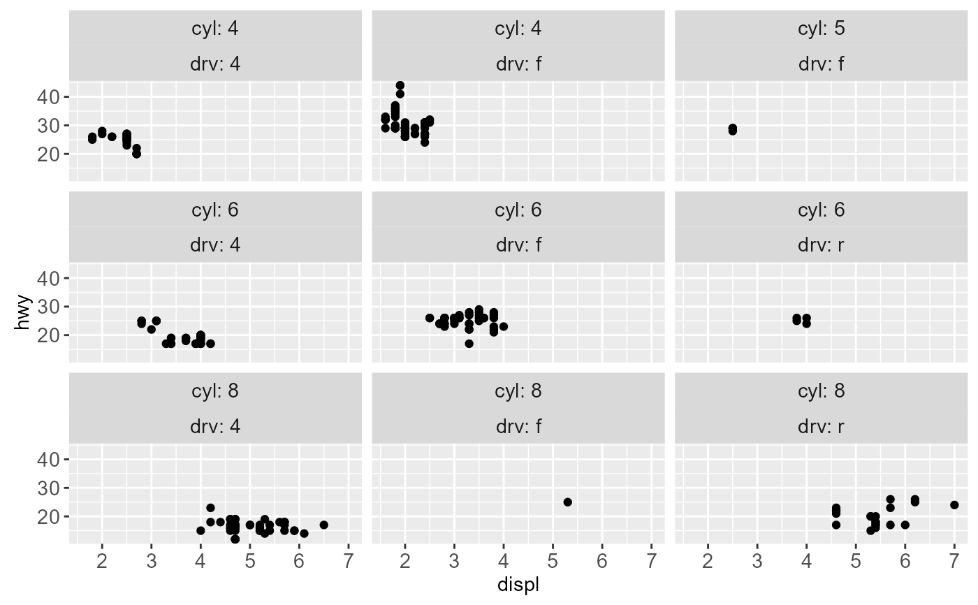
# Use the `labeller` option to control how labels are printed:
ggplot(mpg, aes(displ, hwy)) +
  geom_point() +
  facet_wrap(c("cyl", "drv"), labeller = "label_both")


# To change the order in which the panels appear, change the levels
# of the underlying factor.
mpg$class2 <- reorder(mpg$class, mpg$displ)
ggplot(mpg, aes(displ, hwy)) +
  geom_point() +
  facet_wrap(~class2)


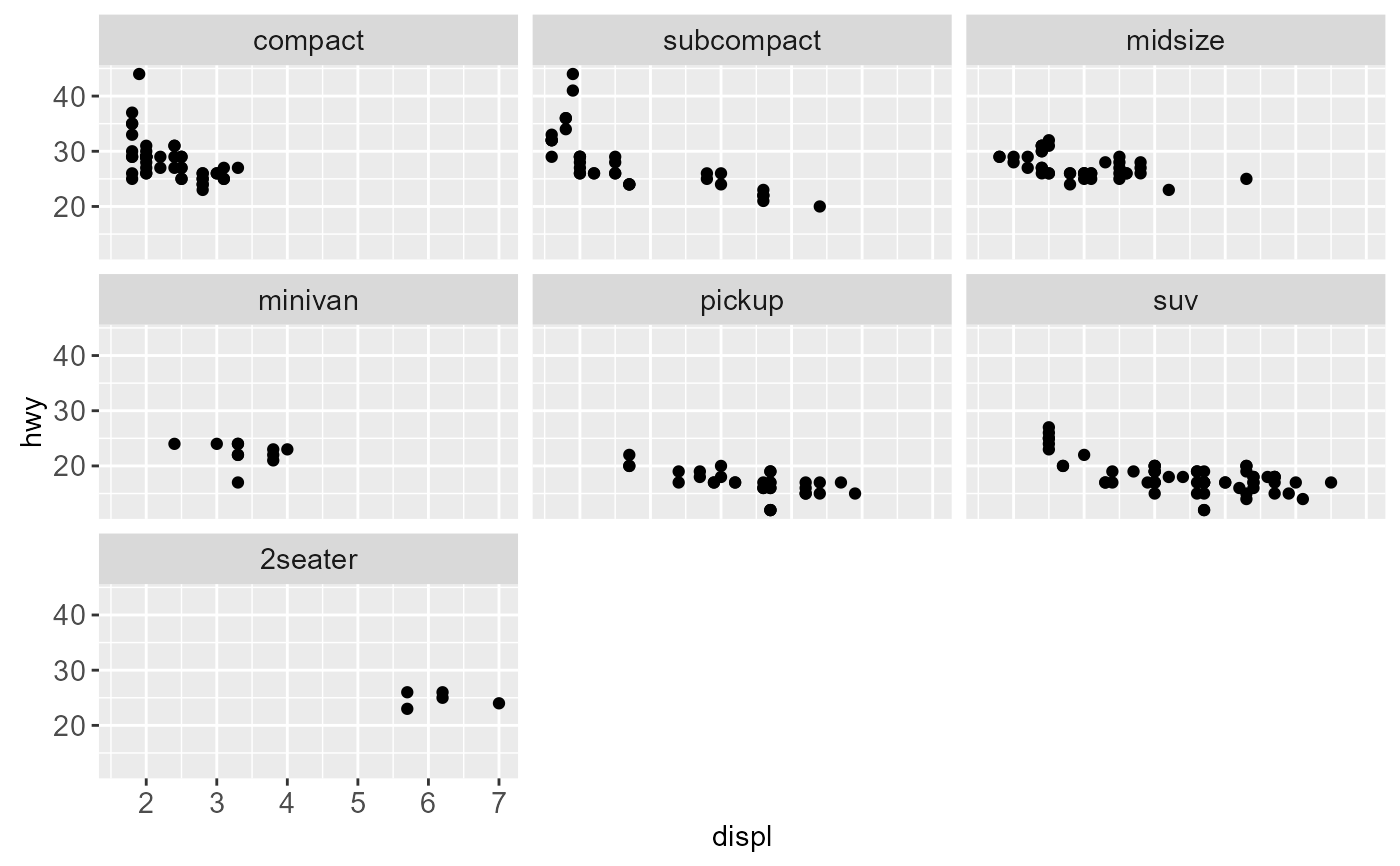# By default, the same scales are used for all panels. You can allow
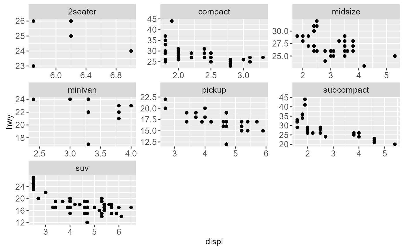
# scales to vary across the panels with the `scales` argument.
# Free scales make it easier to see patterns within each panel, but
# harder to compare across panels.
ggplot(mpg, aes(displ, hwy)) +
  geom_point() +
  facet_wrap(~class, scales = "free")


# To repeat the same data in every panel, simply construct a data frame
# that does not contain the facetting variable.
ggplot(mpg, aes(displ, hwy)) +
  geom_point(data = transform(mpg, class = NULL), colour = "grey85") +
  geom_point() +
  facet_wrap(~class)


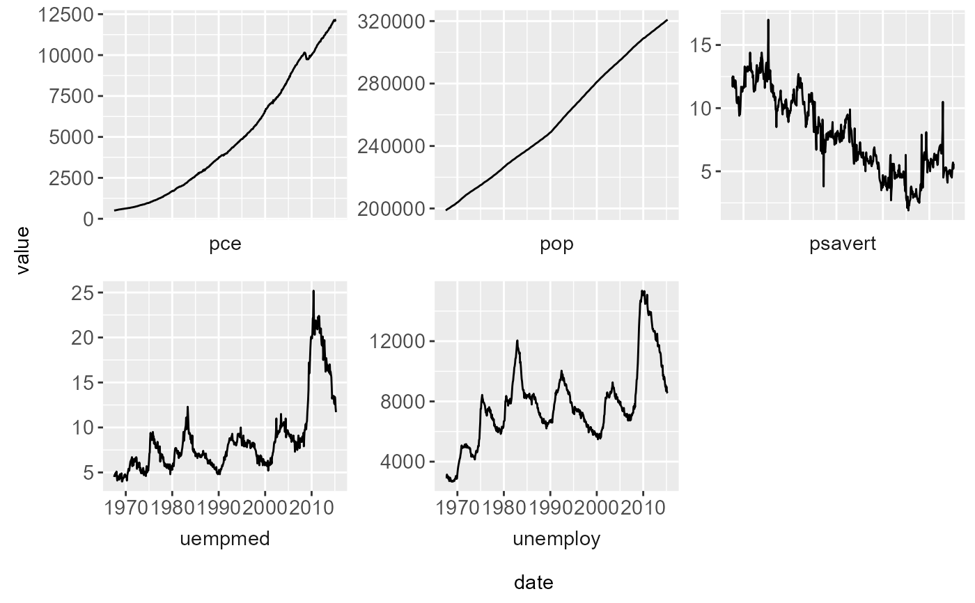
# Use `switch` to display the facet labels near an axis, acting as
# a subtitle for this axis. This is typically used with free scales
# and a theme without boxes around strip labels.
ggplot(economics_long, aes(date, value)) +
  geom_line() +
  facet_wrap(~variable, scales = "free_y", nrow = 2, switch = "x") +
  theme(strip.background = element_blank())

# }